Recently I worked on a PyTorch implementation of the ResNet paper by Kaiming He et al. The paper demonstrates the effect of residual shortcuts in large convolutional neural networks with up to 110 layers and 1.7 million parameters. In this notebook we'll explore the residual shortcut in the extreme minimal setting with just one layer and only 9 parameters. Although not quite as cool as winning ImageNet, as ResNet did in 2016, I hope this helps to clarify residual shortcuts, what they're good for, and how to use them.

Note: If you'd like to execute the code then use the "open in colab" button above, no setup required.

The ResNet architecture enables 110‑layer convolutional networks to outperform 20‑layer networks. The core idea is simple, a stack of 2‑3 convolutional layers circumvented by a 'shortcut' connection from input to output. These 'residual blocks' are themselves stacked together to form the ResNet model, and appear often in machine learning literature.

Resnet Block

Figure 1. A ResNet block and the ResNet architecture

Motivation¶

He et al. start from the observation that 20-layer models out performed 56-layer models on image classification tasks at that time (Fig. 2).

Fig. 2

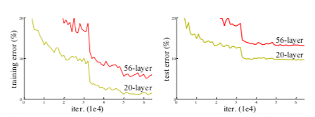
Figure 2. Training error (left) and test error (right) on CIFAR-10 with 20-layer and 56-layer “plain” networks.

Why doesn't the 56-layer model perform at least as well? For example, couldn't the first 20-layers be identical to the smaller model, then the remaining layers just need to output their input. In linear algebra the function that outputs its input is the identity function.

He et al. hypothesised that latter layers in the 56-layer model have a detrimental effect on performance because they struggle to learn how to pass their input through with only fine-grained adjustment. Then they asked, how might we make it easier for convolutional layers to model small changes?

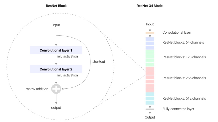
The ResNet solution is to provide a shortcut connection from the input of a layer to its output. The example illustrated in Fig 1. shows a shortcut across two layers.

With a shortcut connection the layer learns the difference, or the residual, between input and output.

$$z = x + f(x) $$

Equation 1.

A simple change but this now means that if the optimal solution is to model the identity function then the layer learns to output a zero matrix for all inputs e.g. $f(x) = 0$. The assumption being that it is easier for a convolutional layer to learn $f(x)$ that returns zero, than it is to learn $f(x)$ that returns $x$. In the authors' words:

"We hypothesize that it is easier to optimize the residual mapping than to optimize the original, unreferenced mapping. To the extreme, if an identity mapping were optimal, it would be easier to push the residual to zero than to fit an identity mapping by a stack of nonlinear layers." - He et al. 2015

Why would it be any easier for a layer to learn a function that maps to zero than it is to learn the identity function? Let's take a closer look.

A minimal example¶

Consider a minimal example, a single convolutional layer that outputs an array of the same shape as its input with kernel size 3, stride 1, padding 1. Our input is a tiny 3x3 grayscale image with a single channel. Assume that the objective is to perform the identity mapping.

With a residual shortcut in place the layer's objective is to output a matrix of zeros irrespective of input. If every weight in the kernel is zero, then every input will be multiplied by zero and so the output must be zero in every position.

Figure 3.

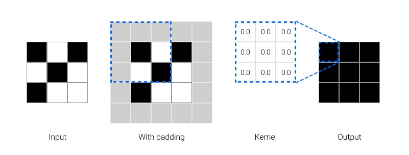
Figure 3. Optimal parameters for a 3x3, stride 1 convolution that maps any input to zero.

Next let's consider the weights needed to perform an identity mapping. In this case the only thing we change is to set the central kernel weight to 1.0. Intuitively the kernel selects the central pixel at each position and ignores all others.

Figure 4.

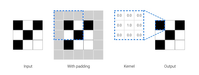
Figure 4. Optimal parameters for a 3x3, stride 1 convolution that maps any input to the unaltered input.

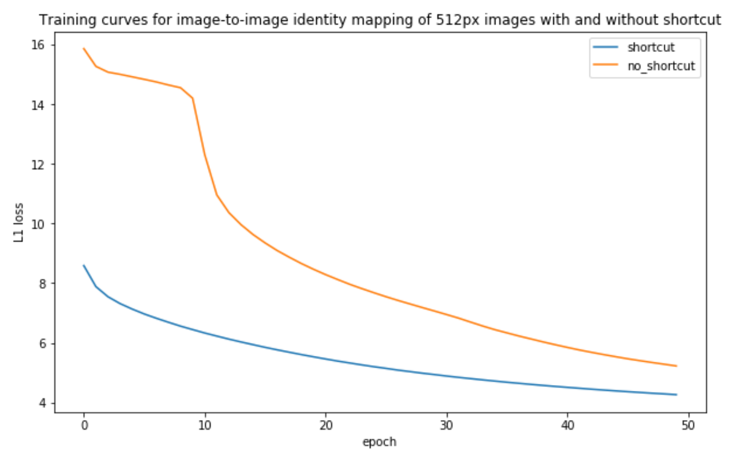
If He's hypothesis is correct we expect that learning the identity objective should be harder than learning the zero objective. It's still not obvious that this is the case but it turns out we can run a very minimal experiment to see for ourselves.

Experiment¶

To test this we'll create the exact same minimal model illustrated in figures 3 & 4, a single convolutional layer with a 3x3 kernel, stride 1, and padding 1. We add a ReLU activation function and initialise the 9 learn-able parameters with Kaiming He's normal initilisation method. Here's our minimal model:

In [1]:

# Import dependencies
import os
import numpy as np
import pandas as pd
import matplotlib.pyplot as plt
import seaborn as sns
import torch
import torch.nn as nn
import torch.nn.functional as F
import torch.optim as optim

In [11]:

class OneConv(nn.Module):
    """Minimal PyTorch model with single convolutional layer"""
    
    def __init__(self, channels):
        """Initialise the model"""
        super().__init__()
        self.conv1 = nn.Conv2d(channels, channels, kernel_size=3, stride=1, 
                               padding=1, bias=False)
        self.relu = nn.ReLU()
        # Initialise weights 
        for m in self.modules():
            if isinstance(m, nn.Conv2d):
                nn.init.kaiming_normal_(m.weight, mode='fan_out', 
                                        nonlinearity='relu')
    
    def forward(self, x):
        """Run a forward pass"""
        z = self.conv1(x)
        z = self.relu(z)
        return z

Next we need a training loop. We use an L1 loss function to measure the absolute difference between the target and the output of the model. With mean reduction across each pixel this is expressed as...

$$l = \frac{\sum_{i=1}^{n}|x_i - y_i|}{n}$$

l: (scalar) loss
n: (scalar) number of samples in dataset
x: (array) input sample
y: (array) target output

The rest is a vanilla backpropagation training loop using an Adam optimiser.

In [4]:

def train(X, Y, epochs):
    """
    Initialises a new model, then trains it for the given number of epochs. 
    The input samples are provide as the array `X` and the targets are 
    provided as an array of the same shape `Y`. The mean loss for each 
    epoch is returned as a list.
    """
    # Initilise model
    model = OneConv(1)
    optimizer = torch.optim.Adam(model.parameters())
    criterion = nn.L1Loss()

    losses = []
    for epoch in range(epochs):
        running_loss = 0.0
        # Train model for an epoch
        for i, x in enumerate(X):
            optimizer.zero_grad()
            z = model(x)
            loss = criterion(z, Y[i])
            loss.backward()
            optimizer.step()
            running_loss += loss.item()

        # Record mean loss for this epoch
        losses.append(running_loss / epochs)
        running_loss = 0.0
    return losses

Now we can run our experiment. We run the experiment multiple times to account for variance due to randomised inputs and weights. For each experiment we generate an array of 200 input samples X. For the identity setting we train a model to map X to X. In the zero setting we train another instance of our model to output zero for each input.

We aggregate the results from each experiment and plot the mean and 95% confidence intervals. (takes ~3 minutes to run on CPU)

In [5]:

n_samples = 200
epochs = 20
experiments = 100

epochs_idx = []
losses = []
experiment = []

# Run each experiment multiple times and accumulate results
for i in range(experiments):
    # Input is random 3x3 matrix
    X = torch.tensor(np.random.random((n_samples, 1, 1, 3, 3)).astype(np.float32))
    # Target is zeros
    Y = torch.tensor(np.zeros((n_samples, 1, 1, 3, 3)).astype(np.float32))

    # Train a model to map input to output, the identity function
    losses += train(X, X, epochs)
    experiment += ['identity' for _ in range(epochs)]
    epochs_idx += list(range(epochs))
    
    # Train a model to map input to zeros
    losses += train(X, Y, epochs)
    experiment += ['zero' for _ in range(epochs)]
    epochs_idx += list(range(epochs))

In [6]:

# Plot results with mean and 95% confidence intervals
df = pd.DataFrame({'epoch': epochs_idx, 
                   'L1_loss': losses, 
                   'experiment': experiment})
plt.figure(figsize=(10, 6))
sns.lineplot(x='epoch', y='L1_loss', hue='experiment', data=df)
plt.axhline(0.01, linestyle='--', color='gray')
plt.title('Comparison of training loss in identity and zero settings.');

In the zero setting the model reduces the L1 loss to below 0.01 (dashed line) in 3.5 epochs, in the identity setting the model takes 10 epochs to achieve this. The wider confidence interval indicates greater variance in the identity setting.

Even in this minimal setting, there is evidence to support He's hypothesis. The model learns a mapping to zero almost three times faster than it learns the identity function.

A less minimal experiment¶

I also ran a similar experiment but with a full 2-layer ResNet block and 512px images as input. More detail on this experiment is available here, and the results are below.

Membrane results

The model with a residual shortcut clearly outperforms the no-shortcut model in this setting too.

Discussion¶

Why do convolutional networks learn the zero mapping more easily than the identity mapping? In the minimal setting there's only two practical differences I can think of:

Weight configuration: In the zero setting the optimal weights are all zero and in the identity setting the central weight should be one and the rest zero.
Target variance: In the identity setting the target is the input which differs at each training step. In the zero setting the target is identical at every step, it is always a zero matrix.

Further investigation is needed. My guess would be that the target variance is the cause.

Summary¶

When the optimal output of a layer is close to the identity function then the residual shortcut ensures that the optimal layer activations are close to zero with reduced variance. We ran a minimal experiment to show that convolutional layers converge faster to a zero mapping (with no variance in target activations), than to an identity mapping (with high variance in target activations).

This suggests that if you can reduce the variance in the target activations of convolutional layers within your model then you can speed up convergence.

Does this apply to nonlinear layers other than convolutions? In settings with other objectives and architectures is the residual the best assumption as to what layers are modeling? If not, do other shortcuts or different techniques for reducing activation variance work better?

In the next post I'll discuss the U-net, another architecture that uses the shortcut technique.

How residual shortcuts speed up learning: a minimal demonstration¶